This notebook presents how to fit a non linear model on a set of data using python. Two kind of algorithms will be presented. First a standard least squares approach using the curve_fit function of scipy.optimize in which we will take into account the uncertainties on the response, that is y. Second a fit with an orthogonal distance regression (ODR) using scipy.odr in which we will take into account the uncertainties on x and y.
Python set up
# manage data and fit
import pandas as pd
import numpy as np

# first part with least squares
from scipy.optimize import curve_fit

# second part about ODR
from scipy.odr import ODR, Model, Data, RealData

# style and notebook integration of the plots
import seaborn as sns
%matplotlib inline
sns.set(style="whitegrid")
Read and plot data
Read the data from a csv file with pandas.
df = pd.read_csv("donnees_exo9.csv", sep=";")
df.head(8) # first 8 lines
| x | y | Dy | |
|---|---|---|---|
| 0 | 0 | 1.371300 | -0.021016 |
| 1 | 1 | 0.747050 | -0.089438 |
| 2 | 2 | 0.587580 | 0.017098 |
| 3 | 3 | 0.510110 | 0.089353 |
| 4 | 4 | 0.424561 | 0.083885 |
| 5 | 5 | 0.394960 | 0.121319 |
| 6 | 6 | 0.157880 | -0.152851 |
| 7 | 7 | 0.223860 | -0.016393 |
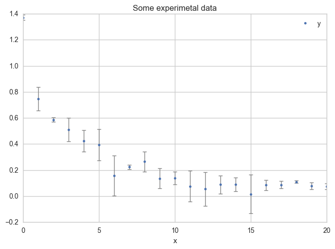
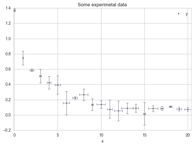
Plot the data with error bars.
ax = df.plot(
    x="x", y="y",
    kind="line", yerr="Dy", title="Some experimental data",
    linestyle="", marker=".",
    capthick=1, ecolor="gray", linewidth=1
)
Fit a model on the data
We want to fit the following model, with parameters, $a$ and $b$, on the above data.
$$f(x) = \ln \dfrac{(a + x)^2}{(x-c)^2}$$
First step : the function
First, we define a function corresponding to the model :
def f_model(x, a, c):
    return pd.np.log((a + x)**2 / (x - c)**2)
Second step : initialisation of parameters
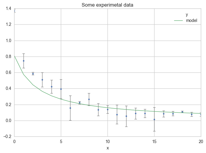
Compute y values for the model with an estimate.
df["model"] = f_model(df["x"], 3, -2)
df.head(8)
| x | y | Dy | model | |
|---|---|---|---|---|
| 0 | 0 | 1.371300 | -0.021016 | 0.810930 |
| 1 | 1 | 0.747050 | -0.089438 | 0.575364 |
| 2 | 2 | 0.587580 | 0.017098 | 0.446287 |
| 3 | 3 | 0.510110 | 0.089353 | 0.364643 |
| 4 | 4 | 0.424561 | 0.083885 | 0.308301 |
| 5 | 5 | 0.394960 | 0.121319 | 0.267063 |
| 6 | 6 | 0.157880 | -0.152851 | 0.235566 |
| 7 | 7 | 0.223860 | -0.016393 | 0.210721 |
Now plot your first estimation of the model.
ax = df.plot(
    x="x", y="y",
    kind="line", yerr="Dy", title="Some experimetal data",
    linestyle="", marker=".",
    capthick=1, ecolor="gray", linewidth=1
)
ax = df.plot(
    x="x", y="model",
    kind="line", ax=ax, linewidth=1
)
Third step : Do the fit
Now we explicitly do the fit with curve_fit using our f_model() function and the initial guess for the parameters. Run help(curve_fit) and read the documentation about the function. curve_fit follow a least-square approach and will minimize :
$$\sum_k \dfrac{\left(f(\text{xdata}_k, \texttt{*popt}) - \text{ydata}_k\right)^2}{\sigma_k^2}$$
help(curve_fit)
popt, pcov = curve_fit(
    f=f_model,       # model function
    xdata=df["x"],   # x data
    ydata=df["y"],   # y data
    p0=(3, -2),      # initial value of the parameters
    sigma=df["Dy"]   # uncertainties on y
)
print(popt)
[ 2.01673012 -1.01484118]
That’s it !
Fourth step : Results of the fit
Parameters are in popt :
a_opt, c_opt = popt
print("a = ", a_opt)
print("c = ", c_opt)
a =  2.01673012047
c =  -1.01484117647
You can compute a standard deviation error from pcov :
perr = np.sqrt(np.diag(pcov))
Da, Dc = perr
print("a = %6.2f +/- %4.2f" % (a_opt, Da))
print("c = %6.2f +/- %4.2f" % (c_opt, Dc))
a =   2.02 +/- 0.06
c =  -1.01 +/- 0.03
You can compute the determination coefficient with :
\begin{equation} R^2 = \frac{\sum_k (y^{calc}_k - \overline{y})^2}{\sum_k (y_k - \overline{y})^2} \end{equation}
R2 = np.sum((f_model(df.x, a_opt, c_opt) - df.y.mean())**2) / np.sum((df.y - df.y.mean())**2)
print("r^2 = %10.6f" % R2)
r^2 = 0.910600
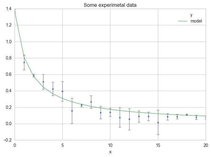
Make a plot
Now, see the results on a plot :
df["model"] = f_model(df.x, a_opt, c_opt)
df.head()
| x | y | Dy | model | |
|---|---|---|---|---|
| 0 | 0 | 1.371300 | -0.021016 | 1.373491 |
| 1 | 1 | 0.747050 | -0.089438 | 0.807266 |
| 2 | 2 | 0.587580 | 0.017098 | 0.573842 |
| 3 | 3 | 0.510110 | 0.089353 | 0.445561 |
| 4 | 4 | 0.424561 | 0.083885 | 0.364284 |
ax = df.plot(
    x="x", y="y",
    kind="line", yerr="Dy", title="Some experimetal data",
    linestyle="", marker=".",
    capthick=1, ecolor="gray", linewidth=1
)
ax = df.plot(
    x="x", y="model",
    kind="line", ax=ax, linewidth=1
)
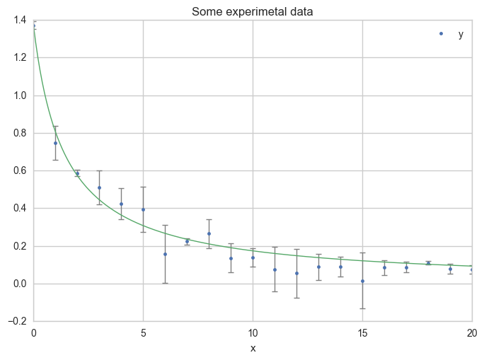
Or using more x values for the model, in order to get a smoother curve :
x = np.linspace(0, 20, 200)
ax = df.plot(
    x="x", y="y",
    kind="line", yerr="Dy", title="Some experimetal data",
    linestyle="", marker=".",
    capthick=1, ecolor="gray", linewidth=1
)
ax.plot(x, f_model(x, a_opt, c_opt), linewidth=1)
Uncertainties on both x and y
x and y are called the independent (or explanatory) and the dependent (the response) variables, respectively. As in the above example, uncertainties are often only take into account on the response variable (y). Here, we will do the same fit but with uncertainties on both x and y variables.
In least square approaches one minimizes, for each value of x, the distance between the response of the model and the data. As you do this for each specific value of x, you cannot include x uncertainties. In order to include them, we will use an orthogonal distance regression approach (ODR). Look at this stackoverflow question from which the following was written.
Add x uncertainties
Add, artificially a random normal uncertainties on x.
nval = len(df)
del df["model"]
Dx = [np.random.normal(0.3, 0.2) for i in range(nval)]
df["Dx"] = Dx
df.head()
| x | y | Dy | Dx | |
|---|---|---|---|---|
| 0 | 0 | 1.371300 | -0.021016 | 0.091596 |
| 1 | 1 | 0.747050 | -0.089438 | -0.015025 |
| 2 | 2 | 0.587580 | 0.017098 | 0.230026 |
| 3 | 3 | 0.510110 | 0.089353 | -0.113324 |
| 4 | 4 | 0.424561 | 0.083885 | 0.232209 |
ax = df.plot(
    x="x", y="y",
    kind="line", yerr="Dy", xerr="Dx",
    title="Some experimetal data",
    linestyle="", marker=".",
    capthick=1, ecolor="gray", linewidth=1
)
Make the fits
1) Define the model
The model function has to be define in a slight different way. The first argument (called beta here) must be the list of the parameters :
def fxy_model(beta, x):
    a, c = beta
    return pd.np.log((a + x)**2 / (x - c)**2)
Define the data and the model
data = RealData(df.x, df.y, df.Dx, df.Dy)
model = Model(fxy_model)
2) Run the algorithms
Two calculations will be donne :
fit_type=2is a least squares approach and consider only y uncertainties.fit_type=0explicit ODR
For each calculation, we make a first iteration and check if convergence is reached with output.info. If not we run at most 100 more time the algorithm while the convergence is not reached.
First you can see that the least squares approach gives the same results as the curve_fit function used above.
odr = ODR(data, model, [3, -2])
odr.set_job(fit_type=2)
lsq_output = odr.run()
print("Iteration 1:")
print("------------")
print("   stop reason:", lsq_output.stopreason)
print("        params:", lsq_output.beta)
print("          info:", lsq_output.info)
print("       sd_beta:", lsq_output.sd_beta)
print("sqrt(diag(cov):", np.sqrt(np.diag(lsq_output.cov_beta)))

# if convergence is not reached, run again the algorithm
if lsq_output.info != 1:
    print("\nRestart ODR till convergence is reached")
    i = 1
    while lsq_output.info != 1 and i < 100:
        print("restart", i)
        lsq_output = odr.restart()
        i += 1
    print("   stop reason:", lsq_output.stopreason)
    print("        params:", lsq_output.beta)
    print("          info:", lsq_output.info)
    print("       sd_beta:", lsq_output.sd_beta)
    print("sqrt(diag(cov):", np.sqrt(np.diag(lsq_output.cov_beta)))
Iteration 1:
------------
   stop reason: ['Sum of squares convergence']
        params: [ 2.01673013 -1.01484118]
          info: 1
       sd_beta: [ 0.0607908   0.03465753]
sqrt(diag(cov): [ 0.08244105  0.04700059]
a_lsq, c_lsq = lsq_output.beta
print("        ODR(lsq)    curve_fit")
print("------------------------------")
print("a = %12.7f %12.7f" % (a_lsq, a_opt))
print("c = %12.7f %12.7f" % (c_lsq, c_opt))
        ODR(lsq)    curve_fit
------------------------------
a =    2.0167301    2.0167301
c =   -1.0148412   -1.0148412
Now the explicit ODR approach with fit_type=0.
odr = ODR(data, model, [3, -2])
odr.set_job(fit_type=0)
odr_output = odr.run()
print("Iteration 1:")
print("------------")
print("   stop reason:", odr_output.stopreason)
print("        params:", odr_output.beta)
print("          info:", odr_output.info)
print("       sd_beta:", odr_output.sd_beta)
print("sqrt(diag(cov):", np.sqrt(np.diag(odr_output.cov_beta)))

# if convergence is not reached, run again the algorithm
if odr_output.info != 1:
    print("\nRestart ODR till convergence is reached")
    i = 1
    while odr_output.info != 1 and i < 100:
        print("restart", i)
        odr_output = odr.restart()
        i += 1
    print("   stop reason:", odr_output.stopreason)
    print("        params:", odr_output.beta)
    print("          info:", odr_output.info)
    print("       sd_beta:", odr_output.sd_beta)
    print("sqrt(diag(cov):", np.sqrt(np.diag(odr_output.cov_beta)))

# Print the results and compare to least square
a_odr, c_odr = odr_output.beta
print("\n        ODR(lsq)    curve_fit     True ODR")
print("--------------------------------------------")
print("a = %12.7f %12.7f %12.7f" % (a_lsq, a_opt, a_odr))
print("c = %12.7f %12.7f %12.7f" % (c_lsq, c_opt, c_odr))
Iteration 1:
------------
   stop reason: ['Sum of squares convergence']
        params: [ 1.94989375 -0.97864174]
          info: 1
       sd_beta: [ 0.11070806  0.0812683 ]
sqrt(diag(cov): [ 0.15857533  0.11640659]

        ODR(lsq)    curve_fit     True ODR
--------------------------------------------
a =    2.0167301    2.0167301    1.9498938
c =   -1.0148412   -1.0148412   -0.9786417
Plot the results
Plot the different results.
x = np.linspace(0, 20, 200)
ax = df.plot(
    x="x", y="y",
    kind="line", yerr="Dy", xerr="Dx",
    title="Some experimetal data",
    linestyle="", marker=".",
    capthick=1, ecolor="gray", linewidth=1
)
ax.plot(x, f_model(x, a_lsq, c_lsq), linewidth=1, label="least square")
ax.plot(x, f_model(x, a_odr, c_odr), linewidth=1, label="ODR")
ax.legend(fontsize=14, frameon=True)
<matplotlib.legend.Legend at 0x1186f59e8>

Although parameters are slightly different, the curves are almost superimposed.