This notebook shows a simple example on how to compute quantities such as energy using LAMMPS from python.
Set up
First of all, you have to install LAMMPS with python bindings in order
to be able to use it from python. A quick test, to know if it works is to
try to import the lammps module from python:
$ > python
Python 3.9.13 | packaged by conda-forge | (main, May 27 2022, 17:01:00)
[Clang 13.0.1 ] on darwin
Type "help", "copyright", "credits" or "license" for more information.
>>> import lammps
>>> lammps.__version__
20210929
In the above output, you can see that I am using python 3.9.13 from
anaconda and I am using the LAMMPS version of September 29, 2021.
To make it works quickly and easily, you can simply install LAMMPS using
conda, preferably in a dedicated environment. The following commands
create a new conda environment, called lmp with python version 3.9. Then
we activate this new environment and add the conda-forge channel to this
specific environment (thanks to the --env option). Then we install
python packages (you can install your prefered ones) and finally we
install LAMMPS.
$ > conda create --name lmp python=3.9
$ > conda activate lmp
$ > conda config --env --add channels conda-forge
$ > conda install numpy matplotlib jupyter pandas
$ > conda install lammps
$ > which python
/Users/my_name/opt/miniconda3/envs/lmp/bin/python
$ > which lmp_serial
/Users/my_name/opt/miniconda3/envs/lmp/bin/lmp_serial
$ > which lmp_mpi
/Users/my_name/opt/miniconda3/envs/lmp/bin/lmp_mpi
$ > lmp_serial
LAMMPS (29 Sep 2021)

$ >
Using conda, the following packages are available (try lmp_serial -h):
Installed packages:

ASPHERE BODY CLASS2 COLLOID COLVARS CORESHELL DIPOLE EXTRA-COMPUTE EXTRA-DUMP
EXTRA-FIX EXTRA-MOLECULE EXTRA-PAIR GRANULAR H5MD KIM KSPACE MANYBODY MC MEAM
MISC ML-IAP ML-SNAP MOLECULE OPT PERI PHONON PLUGIN PYTHON REAXFF REPLICA
RIGID SHOCK SRD USER-VCSGC
If you need other LAMMPS packages or a specific installation to manage efficiency, you have to consider compiling lammps by yourself.
import os
import lammps
import numpy as np
import pandas as pd
Run a LAMMPS calculation
To run a LAMMPS calculation from python you need the same information as if you intend to run LAMMPS classically. If you look for an API which fill in an input file with default parameters for you, starting only from your system, you may try ASE (atomic simulation environment).
A Methane box
Here we run simulation on a methane box using a Lenard Jones potential. Let’s write a LAMMPS input file in which you fill a box with 2000 methane particles using the TraPPE potential. The syntax is the same as the one of a classic LAMMPS input.
methane_inp = """# LAMMPS input file for Methane

units real
atom_style atomic

region myRegion block 0. 400. 0. 400. 0. 400. units box
create_box 1 myRegion
create_atoms 1 random 2000 03042019 myRegion

# LJ Methane: TraPPE potential
# eps / k_B = 148.0
# eps = 148.0 * k_B * N_a * 1e-3 / 4.184
#
pair_style lj/cut 14.0
pair_coeff   1   1    0.2941    3.730
pair_modify shift no mix arithmetic tail yes
mass 1 16.04

run_style verlet
neighbor 2.0 bin
neigh_modify delay 10

timestep 2.0
thermo_style multi
thermo 200
"""
In order to run the calculations, you have to initialize the lammps object
and execute LAMMPS commands through it.
# setup the lammps object and reduce verbosity
# lmp = lammps.lammps(cmdargs=["-log", "none", "-nocite"])
lmp = lammps.lammps(cmdargs=["-nocite"])
# load the initialization commands
lmp.commands_string(methane_inp)
LAMMPS (29 Sep 2021)
OMP_NUM_THREADS environment is not set. Defaulting to 1 thread. (src/comm.cpp:98)
  using 1 OpenMP thread(s) per MPI task
Created orthogonal box = (0.0000000 0.0000000 0.0000000) to (400.00000 400.00000 400.00000)
  1 by 1 by 1 MPI processor grid
Created 2000 atoms
  using lattice units in orthogonal box = (0.0000000 0.0000000 0.0000000) to (400.00000 400.00000 400.00000)
  create_atoms CPU = 0.000 seconds
The simulations is still alive and you can for exemple, run one NVE step just to compute energy.
lmp.commands_list([
    "fix NVE all nve",
    "run 0"
])
Neighbor list info ...
  update every 1 steps, delay 10 steps, check yes
  max neighbors/atom: 2000, page size: 100000
  master list distance cutoff = 16
  ghost atom cutoff = 16
  binsize = 8, bins = 50 50 50
  1 neighbor lists, perpetual/occasional/extra = 1 0 0
  (1) pair lj/cut, perpetual
      attributes: half, newton on
      pair build: half/bin/atomonly/newton
      stencil: half/bin/3d
      bin: standard
Setting up Verlet run ...
  Unit style    : real
  Current step  : 0
  Time step     : 2
Per MPI rank memory allocation (min/avg/max) = 3.820 | 3.820 | 3.820 Mbytes
---------------- Step        0 ----- CPU =      0.0000 (sec) ----------------
TotEng   =      7136.6806 KinEng   =         0.0000 Temp     =         0.0000
PotEng   =      7136.6806 E_bond   =         0.0000 E_angle  =         0.0000
E_dihed  =         0.0000 E_impro  =         0.0000 E_vdwl   =      7136.6806
E_coul   =         0.0000 E_long   =         0.0000 Press    =        31.0191
Loop time of 1.47699e-06 on 1 procs for 0 steps with 2000 atoms

135.4% CPU use with 1 MPI tasks x 1 OpenMP threads

MPI task timing breakdown:
Section |  min time  |  avg time  |  max time  |%varavg| %total
---------------------------------------------------------------
Pair    | 0          | 0          | 0          |   0.0 |  0.00
Neigh   | 0          | 0          | 0          |   0.0 |  0.00
Comm    | 0          | 0          | 0          |   0.0 |  0.00
Output  | 0          | 0          | 0          |   0.0 |  0.00
Modify  | 0          | 0          | 0          |   0.0 |  0.00
Other   |            | 1.477e-06  |            |       |100.00

Nlocal:        2000.00 ave        2000 max        2000 min
Histogram: 1 0 0 0 0 0 0 0 0 0
Nghost:        540.000 ave         540 max         540 min
Histogram: 1 0 0 0 0 0 0 0 0 0
Neighs:        557.000 ave         557 max         557 min
Histogram: 1 0 0 0 0 0 0 0 0 0

Total # of neighbors = 557
Ave neighs/atom = 0.27850000
Neighbor list builds = 0
Dangerous builds = 0
etotal_0 = lmp.get_thermo("etotal")
print(f"E_total = {etotal_0:.2f} kcal.mol-1")
E_total = 7136.68 kcal.mol-1
Let’s now run a minimization and get back energies:
lmp.commands_string("minimize 1.0e-4 1.0e-6 1000 1000")
etotal_min = lmp.get_thermo("etotal")
WARNING: Using 'neigh_modify every 1 delay 0 check yes' setting during minimization (src/min.cpp:188)
Setting up cg style minimization ...
  Unit style    : real
  Current step  : 0
Per MPI rank memory allocation (min/avg/max) = 4.945 | 4.945 | 4.945 Mbytes
---------------- Step        0 ----- CPU =      0.0000 (sec) ----------------
TotEng   =      7136.6806 KinEng   =         0.0000 Temp     =         0.0000
PotEng   =      7136.6806 E_bond   =         0.0000 E_angle  =         0.0000
E_dihed  =         0.0000 E_impro  =         0.0000 E_vdwl   =      7136.6806
E_coul   =         0.0000 E_long   =         0.0000 Press    =        31.0191
---------------- Step      200 ----- CPU =      0.0202 (sec) ----------------
TotEng   =       -32.3026 KinEng   =         0.0000 Temp     =         0.0000
PotEng   =       -32.3026 E_bond   =         0.0000 E_angle  =         0.0000
E_dihed  =         0.0000 E_impro  =         0.0000 E_vdwl   =       -32.3026
E_coul   =         0.0000 E_long   =         0.0000 Press    =        -0.0030
---------------- Step      400 ----- CPU =      0.0406 (sec) ----------------
TotEng   =       -44.6657 KinEng   =         0.0000 Temp     =         0.0000
PotEng   =       -44.6657 E_bond   =         0.0000 E_angle  =         0.0000
E_dihed  =         0.0000 E_impro  =         0.0000 E_vdwl   =       -44.6657
E_coul   =         0.0000 E_long   =         0.0000 Press    =        -0.0017
---------------- Step      531 ----- CPU =      0.0538 (sec) ----------------
TotEng   =       -51.8396 KinEng   =         0.0000 Temp     =         0.0000
PotEng   =       -51.8396 E_bond   =         0.0000 E_angle  =         0.0000
E_dihed  =         0.0000 E_impro  =         0.0000 E_vdwl   =       -51.8396
E_coul   =         0.0000 E_long   =         0.0000 Press    =        -0.0013
Loop time of 0.0537888 on 1 procs for 531 steps with 2000 atoms

99.6% CPU use with 1 MPI tasks x 1 OpenMP threads

Minimization stats:
  Stopping criterion = energy tolerance
  Energy initial, next-to-last, final =
      7136.68060804696  -51.8346790636406  -51.8396011281685
  Force two-norm initial, final = 42230.019 0.14334973
  Force max component initial, final = 22010.982 0.072526514
  Final line search alpha, max atom move = 1.0000000 0.072526514
  Iterations, force evaluations = 531 546

MPI task timing breakdown:
Section |  min time  |  avg time  |  max time  |%varavg| %total
---------------------------------------------------------------
Pair    | 0.0094555  | 0.0094555  | 0.0094555  |   0.0 | 17.58
Neigh   | 0.012789   | 0.012789   | 0.012789   |   0.0 | 23.78
Comm    | 0.0027082  | 0.0027082  | 0.0027082  |   0.0 |  5.03
Output  | 9.0669e-05 | 9.0669e-05 | 9.0669e-05 |   0.0 |  0.17
Modify  | 0          | 0          | 0          |   0.0 |  0.00
Other   |            | 0.02875    |            |       | 53.44

Nlocal:        2000.00 ave        2000 max        2000 min
Histogram: 1 0 0 0 0 0 0 0 0 0
Nghost:        538.000 ave         538 max         538 min
Histogram: 1 0 0 0 0 0 0 0 0 0
Neighs:        553.000 ave         553 max         553 min
Histogram: 1 0 0 0 0 0 0 0 0 0

Total # of neighbors = 553
Ave neighs/atom = 0.27650000
Neighbor list builds = 38
Dangerous builds = 0
print(f"E_total after minimization {etotal_min:.2f} kcal.mol-1")
print(f"Delta E_total = {etotal_min - etotal_0:.2f} kcal.mol-1")
E_total after minimization -51.84 kcal.mol-1
Delta E_total = -7188.52 kcal.mol-1
Let’s now set up a short NVT simulations.
lmp.commands_list([
    "velocity all create 300. 03042019 dist gaussian mom yes rot yes",
    "fix NVT all nvt temp 300. 300. $(100.0 * dt)",
    "dump trj all custom 10 traj.lammpstrj id type element x y z",
    "run 1000",
])
WARNING: One or more atoms are time integrated more than once (src/modify.cpp:281)
Setting up Verlet run ...
  Unit style    : real
  Current step  : 531
  Time step     : 2
Per MPI rank memory allocation (min/avg/max) = 3.820 | 3.820 | 3.820 Mbytes
---------------- Step      531 ----- CPU =      0.0000 (sec) ----------------
TotEng   =      1735.7522 KinEng   =      1787.5918 Temp     =       300.0000
PotEng   =       -51.8396 E_bond   =         0.0000 E_angle  =         0.0000
E_dihed  =         0.0000 E_impro  =         0.0000 E_vdwl   =       -51.8396
E_coul   =         0.0000 E_long   =         0.0000 Press    =         1.2755
---------------- Step      600 ----- CPU =      0.0176 (sec) ----------------
TotEng   =      1741.6774 KinEng   =      1774.6823 Temp     =       297.8335
PotEng   =       -33.0049 E_bond   =         0.0000 E_angle  =         0.0000
E_dihed  =         0.0000 E_impro  =         0.0000 E_vdwl   =       -33.0049
E_coul   =         0.0000 E_long   =         0.0000 Press    =         1.2303
---------------- Step      800 ----- CPU =      0.0690 (sec) ----------------
TotEng   =      1844.5829 KinEng   =      1860.1245 Temp     =       312.1727
PotEng   =       -15.5416 E_bond   =         0.0000 E_angle  =         0.0000
E_dihed  =         0.0000 E_impro  =         0.0000 E_vdwl   =       -15.5416
E_coul   =         0.0000 E_long   =         0.0000 Press    =         1.3273
---------------- Step     1000 ----- CPU =      0.1194 (sec) ----------------
TotEng   =      1752.7727 KinEng   =      1769.8605 Temp     =       297.0243
PotEng   =       -17.0878 E_bond   =         0.0000 E_angle  =         0.0000
E_dihed  =         0.0000 E_impro  =         0.0000 E_vdwl   =       -17.0878
E_coul   =         0.0000 E_long   =         0.0000 Press    =         1.2571
---------------- Step     1200 ----- CPU =      0.1686 (sec) ----------------
TotEng   =      1795.0916 KinEng   =      1812.1438 Temp     =       304.1204
PotEng   =       -17.0522 E_bond   =         0.0000 E_angle  =         0.0000
E_dihed  =         0.0000 E_impro  =         0.0000 E_vdwl   =       -17.0522
E_coul   =         0.0000 E_long   =         0.0000 Press    =         1.2822
---------------- Step     1400 ----- CPU =      0.2176 (sec) ----------------
TotEng   =      1714.2492 KinEng   =      1731.4279 Temp     =       290.5744
PotEng   =       -17.1787 E_bond   =         0.0000 E_angle  =         0.0000
E_dihed  =         0.0000 E_impro  =         0.0000 E_vdwl   =       -17.1787
E_coul   =         0.0000 E_long   =         0.0000 Press    =         1.2300
---------------- Step     1531 ----- CPU =      0.2516 (sec) ----------------
TotEng   =      1774.7488 KinEng   =      1790.4497 Temp     =       300.4796
PotEng   =       -15.7009 E_bond   =         0.0000 E_angle  =         0.0000
E_dihed  =         0.0000 E_impro  =         0.0000 E_vdwl   =       -15.7009
E_coul   =         0.0000 E_long   =         0.0000 Press    =         1.2755
Loop time of 0.251606 on 1 procs for 1000 steps with 2000 atoms

Performance: 686.789 ns/day, 0.035 hours/ns, 3974.475 timesteps/s
96.1% CPU use with 1 MPI tasks x 1 OpenMP threads

MPI task timing breakdown:
Section |  min time  |  avg time  |  max time  |%varavg| %total
---------------------------------------------------------------
Pair    | 0.013527   | 0.013527   | 0.013527   |   0.0 |  5.38
Neigh   | 0.020657   | 0.020657   | 0.020657   |   0.0 |  8.21
Comm    | 0.0046987  | 0.0046987  | 0.0046987  |   0.0 |  1.87
Output  | 0.17079    | 0.17079    | 0.17079    |   0.0 | 67.88
Modify  | 0.038092   | 0.038092   | 0.038092   |   0.0 | 15.14
Other   |            | 0.00384    |            |       |  1.53

Nlocal:        2000.00 ave        2000 max        2000 min
Histogram: 1 0 0 0 0 0 0 0 0 0
Nghost:        516.000 ave         516 max         516 min
Histogram: 1 0 0 0 0 0 0 0 0 0
Neighs:        596.000 ave         596 max         596 min
Histogram: 1 0 0 0 0 0 0 0 0 0

Total # of neighbors = 596
Ave neighs/atom = 0.29800000
Neighbor list builds = 62
Dangerous builds = 0
If you want to deal with the coordinates of the methane molecules you can extract them in a numpy array:
coords = lmp.numpy.extract_atom("x")
print(coords.shape)
(2000, 3)
coords[:10, :]
array([[149.58560661,   2.41219752,   2.57614008],
       [333.9610746 ,   9.95530239,  21.59438813],
       [329.78342159,  29.97893778, 396.44644249],
       [321.08765039,  32.5780972 ,   0.49664071],
       [378.08752875,  45.88949262, 391.57425535],
       [160.10914446,  83.14035611,  13.87252111],
       [300.41131912,  72.64511171,  24.14922672],
       [326.19055095,  75.11154388, 396.45508269],
       [ 58.12894298, 107.25813816, 391.26395367],
       [157.61119189, 113.33277942,   9.00796178]])
At the end, close the LAMMPS execution:
lmp.close()
Total wall time: 0:00:19
Visualization
One can try to watch the LAMMPS trajectory using a combination of the mdtraj
and nglview modules.
Set up topology
If you have a pdb file of your system, it can be used as a topology. Else, you have to create the object by hand.
import mdtraj
import nglview as nv
# make topology by hand ...
top = mdtraj.Topology()
chain = top.add_chain()
n_atoms = 2000
for iat in range(n_atoms):
    res = top.add_residue(f"Me{iat}", chain=chain)
    top.add_atom(name="C", element=mdtraj.element.carbon, residue=res, serial=iat)
Load the trajectory from file and get a visualization with nglview.
traj = mdtraj.load_lammpstrj("traj.lammpstrj", top=top)
view = nv.show_mdtraj(traj)
view.clear()
view.center()
view.add_spacefill(radius=20.0)
view.add_unitcell()
view
NGLWidget(max_frame=99)
# view.render_image()
view._display_image()

Methanol PES
Here is an example on how to use LAMMPS in order to compute the energy of your system, considering a given methodology (molecular mechanics here) and a series of molecular structures.
The system consists in a methanol molecule in vacuum and the corresponding
data file is methanol.data.
In the following input we simply read this data file and define the force
field. As we will not do any simulation later, Verlet scheme and neighbor list
options are not specified and default values are used. Of course,
atom_style and force fields options must be consistent with the data file.
methanol_inp = """# LAMMPS input file for Methanol

units real
atom_style full
boundary  f f f

bond_style harmonic
angle_style harmonic
dihedral_style opls
pair_style      lj/cut/coul/cut 14

read_data methanol.data

# LJ: OPLS
# energy = kcal/mol
# distance = angstrom
pair_coeff        1        1    0.0660     3.5000
pair_coeff        2        2    0.0300     2.5000
pair_coeff        3        3    0.1700     3.1200
pair_coeff        4        4    0.0000     0.0000
pair_modify shift no mix geometric
special_bonds amber

fix NVE all nve
"""
One single calculation
Again, we create the lammps object. Here we reduce output and redirect
stdout to devnull.
lmp.close()
lmp = lammps.lammps(cmdargs=["-log", "none", "-screen", os.devnull,  "-nocite"])
lmp.commands_string(methanol_inp)
Let’s make an energy calculation and output energy quantities.
lmp.command("run 0")
for energy in ["etotal", "evdwl", "ecoul", "ebond", "eangle", "edihed"]:
    print(f"{energy:8s} {lmp.get_thermo(energy):10.4f} kcal.mol-1")
etotal       7.5410 kcal.mol-1
evdwl        0.0000 kcal.mol-1
ecoul        3.1738 kcal.mol-1
ebond        4.2671 kcal.mol-1
eangle       0.1001 kcal.mol-1
edihed       0.0000 kcal.mol-1
It’s possible to extract the last (current) geometry of the calculation and reconstruct
the molecule. Note that, in this particular case, with run 0 the geometry is the same as the
input one.
Remember also, that in LAMMPS, by default, atoms are not sorted (if you perform several steps). It is thus safer to get atom ids.
Here we use the numpy property of the lammps object to get numpy arrays (more convenient) instead of pointers.
coords = lmp.numpy.extract_atom("x")
print("coords\n", coords)

ids = lmp.numpy.extract_atom("id")
print("atom ids", ids)

i_types = lmp.numpy.extract_atom("type")
print("atom types", i_types)

elements = ["C", "H", "O", "H"]
dict_types = {i: el for i, el in enumerate(elements, 1)}

# TODO: sort by id if needed
print(f"\n{'el':2s} {'id':>4s}{'x':>12s} {'y':>12s} {'z':>12s}")
for iat in range(lmp.get_natoms()):
    specie = dict_types[i_types[iat]]
    xyz = coords[iat]
    line =  f"{specie:2s} {ids[iat]:4d}"
    line += " ".join([f"{x:12.6f}" for x in xyz])
    print(line)
coords
 [[ 0.       0.       0.     ]
 [ 0.63     0.63     0.63   ]
 [-0.63    -0.63     0.63   ]
 [ 0.63    -0.63    -0.63   ]
 [-0.86603  0.86603 -0.86603]
 [-0.28871  1.4434  -1.4434 ]]
atom ids [1 2 3 4 5 6]
atom types [1 2 2 2 3 4]

el   id           x            y            z
C     1    0.000000     0.000000     0.000000
H     2    0.630000     0.630000     0.630000
H     3   -0.630000    -0.630000     0.630000
H     4    0.630000    -0.630000    -0.630000
O     5   -0.866030     0.866030    -0.866030
H     6   -0.288710     1.443400    -1.443400
lmp.close()
PES calculations
Hereafter, we compute the energy on a series of geometries read from an xyz file.
First we read the coordinates in the scan.allxyz file.
It consists in 73 geometries of methanol along the dihedral angle H-O-C-H.
scan_coords = list()
with open("scan.allxyz", "r") as f:
    chunks = f.read().split(">")
    for chunk in chunks:
        lines = chunk.strip().split("\n")
        coords = list()
        for line in lines[2:]:
            coords.append(line.split()[1:])
        scan_coords.append(coords)
scan_coords = np.array(scan_coords, dtype=np.float64)

n_geo, n_atoms, n_dim = scan_coords.shape
print(n_geo, n_atoms, n_dim)
73 6 3
Now, again we initialize the LAMMPS object and load the force fields information as previously.
lmp.close()
lmp = lammps.lammps(cmdargs=["-log", "none", "-screen", os.devnull,  "-nocite"])
lmp.commands_string(methanol_inp)
We write a loop over the geometries read in the the scan.allxyz file. The
atoms’ coordinates are accessible from a pointer by interacting with the current
LAMMPS execution.
Hereafter, we get back the pointer in the p_coords variable. Then, in a loop,
the coordinates are updated and the energy is computed as done previously for
one single geometry.
Thanks to the default thermo variables, for each geometry we store the different
energy components in a dictionary.
# get the pointers on coordinates => used to update geometry
p_coords = lmp.extract_atom("x")

scan_data = list()
dihedral = 0
for step_coords in scan_coords:
    dihedral += 5.0

    # update coordinates
    # p_coords is not a numpy array but a double C pointer
    for iat in range(n_atoms):
        p_coords[iat][0], p_coords[iat][1], p_coords[iat][2] = step_coords[iat]

    # compute energy
    lmp.command("run 0")

    # get back results
    step_data = dict(dihedral=dihedral)
    for energy in ["etotal", "evdwl", "ecoul", "ebond", "eangle", "edihed"]:
        step_data[energy] = lmp.get_thermo(energy)

    scan_data.append(step_data)
lmp.close()
We gather data in a pandas DataFrame in combination with QM energies
associated to the geometries. The energies are available in the
scan.qm.dat file.
df = pd.DataFrame(scan_data)
df.set_index("dihedral", inplace=True)
df.etotal -= df.etotal.min()
df.head()
| etotal | evdwl | ecoul | ebond | eangle | edihed | |
|---|---|---|---|---|---|---|
| dihedral | ||||||
| 5.0 | 0.853286 | 0.0 | 3.276409 | 0.082618 | 0.205623 | 1.055928 |
| 10.0 | 0.838037 | 0.0 | 3.276421 | 0.083220 | 0.207423 | 1.038266 |
| 15.0 | 0.794073 | 0.0 | 3.276481 | 0.085447 | 0.212537 | 0.986901 |
| 20.0 | 0.725481 | 0.0 | 3.276334 | 0.089648 | 0.221138 | 0.905654 |
| 25.0 | 0.637719 | 0.0 | 3.275813 | 0.095966 | 0.233131 | 0.800102 |
qm_df = pd.read_csv(
    "scan.qm.dat",
    index_col=0,
    delim_whitespace=True,
    names=["dihedral", "QM"]
)
qm_df -= qm_df.QM.min()
qm_df *= 627.5095  # Hartree -> kcal.mol-1
qm_df.head()
| QM | |
|---|---|
| dihedral | |
| 0.0 | 1.512185 |
| 5.0 | 1.482642 |
| 10.0 | 1.403670 |
| 15.0 | 1.283351 |
| 20.0 | 1.131619 |
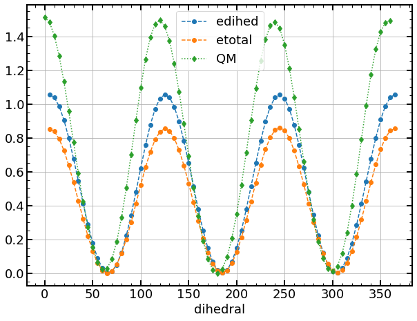
Now depending on what you want to do, you can compare the contributions of each energy to the total energy and compare them to the QM energy.
Here, in the case of OPLS force field of a dihedral angle, considering the height of the energy barriers, differences are smaller than the expected accuracy.
ax = df.plot(y=["edihed", "etotal"], marker="o", ls="--")
ax = qm_df.plot(ax=ax, marker="d", ls=":")