This notebook presents and compares several ways to compute the Kernel Density Estimation (KDE) of the probability density function (PDF) of a random variable. KDE plots are available in usual python data analysis and visualization packages such as pandas or seaborn. These packages relies on statistics packages to compute the KDE and this notebook will present you how to compute the KDE either by hand or using scipy.
For a more complete reading about KDE, you should read this article.
%matplotlib inline
import numpy as np
import scipy as sp
from scipy.stats import gaussian_kde
from scipy.stats import norm
import pandas as pd
import seaborn as sns

import matplotlib.pyplot as plt
import matplotlib.patches as mpatches
plt.rcParams["figure.figsize"] = (9, 6)
plt.rcParams["font.size"] = 18

# just for fun
# plt.xkcd(scale=.5, length=50);
The results strongly depend on the version of the used packages. For example, seaborn will compute the kde using either scipy or statsmodels and depending on the scipy version, the meaning of the kde width is not the same. Hereafter are the package versions used in this notebook.
print(f"Numpy: {np.__version__}")
print(f"Scipy: {sp.__version__}")
print(f"Pandas: {pd.__version__}")
print(f"Seaborn: {sns.__version__}")
Numpy: 1.16.2
Scipy: 1.2.1
Pandas: 0.24.2
Seaborn: 0.9.0
Sample
This is a data sample that will we used in this notebook.
data = [-20.31275116, -18.3594738, -18.3553103, -14.18406452, -11.67305,
        -11.38179997, -11.3761126, -10.6904519, -10.68305023, -10.34148,
         -8.75222277,  -8.7498553, -6.00130727,   1.45761078,   1.77479,
          1.78314794,   2.6612791]
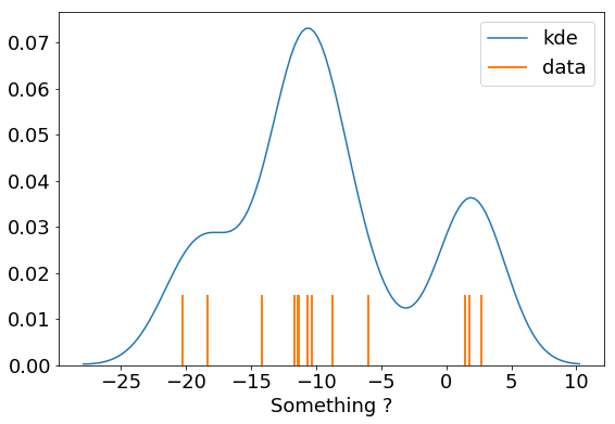
seaborn is a good option to get a quick view of the data. You can plot the data as a rugplot and the KDE. In seaborn the default kernel is a gaussian kernel.
sns.distplot(data, hist=False, rug=True,
             axlabel="Something ?",
             kde_kws=dict(label="kde"),
             rug_kws=dict(height=.2, linewidth=2, color="C1", label="data"))
plt.legend();
Compute the gaussian KDE by hands
A gaussian KDE is computed from a sum of normal functions of a defined width. It could be computed as follow:
def my_kde(data, width=1, gridsize=100, normalized=True, bounds=None):
    """
    Compute the gaussian KDE from the given sample.

    Args:
        data (array or list): sample of values
        width (float): width of the normal functions
        gridsize (int): number of grid points on which the kde is computed
        normalized (bool): if True the KDE is normalized (default)
        bounds (tuple): min and max value of the kde

    Returns:
        The grid and the KDE
    """
    # boundaries
    if bounds:
        xmin, xmax = bounds
    else:
        xmin = min(data) - 3 * width
        xmax = max(data) + 3 * width

    # grid points
    x = np.linspace(xmin, xmax, gridsize)

    # compute kde
    kde = np.zeros(gridsize)
    for val in data:
        kde += norm.pdf(x, loc=val, scale=width)

    # normalized the KDE
    if normalized:
        kde /= sp.integrate.simps(kde, x)

    return x, kde
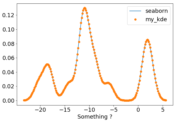
Using our function, the KDE is computed as:
x, kde = my_kde(data, gridsize=200)
Now we can compare with the KDE obtained from seaborn. The gaussian kernel being the default, we have to give to seaborn the same band width, that is 1. here, using the bw keyword.
ax = sns.distplot(data, hist=False, axlabel="Something ?",
                  kde_kws=dict(gridsize=200, bw=1, label="seaborn"))
ax.plot(x, kde, "o", label="my_kde")
plt.legend();
Compute the gaussian KDE with scipy
Using available methods from reliable packages such as scipy is always a better option. In addition to save time the functions are generally more efficient and less buggy.
Here we will use the gaussian_kde class from the scipy.stats module.
# KDE instance
bw = 1. / np.std(data)
g_kde = gaussian_kde(dataset=data, bw_method=bw)

# compute KDE
gridsize = 200
g_x = np.linspace(-24, 6, gridsize)
g_kde_values = g_kde(g_x)
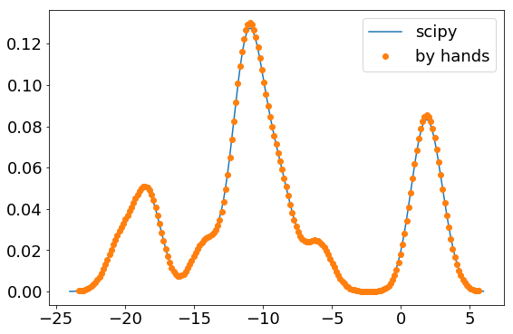
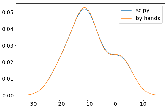
Now we can compare with our previous KDE computed by hands.
Remark: In scipy, the bandwidth is scaled by the covariance of the input data, that is the standard deviation here. Thus, for comparison, the bandwidth is divided by the standard deviation.
plt.plot(g_x, g_kde_values, label="scipy")
plt.plot(x, kde, "o", label="by hands")
plt.legend();
There are several methods embedded in the gaussian_kde class in order to integrate or sample using the new kernel.
Depending on the bw_method argument, the class can compute an estimator of the bandwidth which could be obtained from a class attribute.
g_kde = gaussian_kde(dataset=data, bw_method="scott")
print(f"Band width: {g_kde.factor}")
g_kde = gaussian_kde(dataset=data, bw_method="silverman")
print(f"Band width: {g_kde.factor}")
Band width: 0.5674272856715801
Band width: 0.6010325090449528
If you want to use this new value in our my_kde() functions, don’t forget to scaled the bandwidth by the standard deviation of the input data.
# compute KDE value from gaussian_kde instance
g_kde = gaussian_kde(dataset=data, bw_method="silverman")
g_kde_values = g_kde(g_x)
# our functions with the computed bandwidth
x, kde = my_kde(data, width=g_kde.factor * np.std(data), gridsize=200)
# plot
plt.plot(g_x, g_kde_values, label="scipy")
plt.plot(x, kde, label="by hands")
plt.legend();
About performances
Hereafter is a comparison of the performances of our functions and scipy gaussian_kde class. You can see that scipy is three times faster.
%timeit x, kde = my_kde(data, width=g_kde.factor, gridsize=200)
2.2 ms ± 190 µs per loop (mean ± std. dev. of 7 runs, 1000 loops each)
%%timeit
# KDE instance
g_kde = gaussian_kde(dataset=data, bw_method=0.14)

# compute KDE
gridsize = 200
g_x = np.linspace(-24, 6, gridsize)
g_kde_values = g_kde(g_x)
755 µs ± 70.6 µs per loop (mean ± std. dev. of 7 runs, 1000 loops each)
Comparisons
Now, let us compare the KDE obtained from either our functions, scipy, seaborn or pandas.
df = pd.DataFrame(data, columns=["data"])
df.head()
| data | |
|---|---|
| 0 | -20.312751 |
| 1 | -18.359474 |
| 2 | -18.355310 |
| 3 | -14.184065 |
| 4 | -11.673050 |
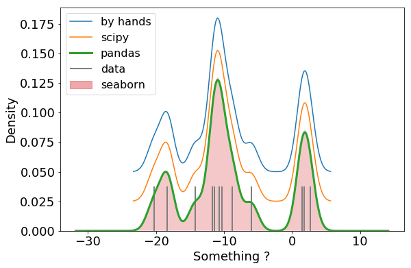
Note in the following cell that in seaborn (with gaussian kernel) the meaning of the bandwidth is the same as the one in our function (the width of the normal functions summed to obtain the KDE). As pandas uses scipy the meaning of the band width is different and for comparison, using scipy or pandas, you have to scale the bandwidth by the standard deviation.
In the plot below, the KDE computed by hands or using scipy are shifted vertically for a better comparison.
# bandwidth
bw = 1.
bw_sp = bw / np.std(data)

# KDE from our function
ax = plt.subplot()
x, kde = my_kde(data, width=bw, gridsize=200)
ax.plot(x, kde + 0.05, label="by hands")

# scipy
g_kde = gaussian_kde(dataset=data, bw_method=bw_sp)
g_kde_values = g_kde(x)
ax.plot(x, g_kde_values + 0.025, label="scipy")

# pandas
df.data.plot.kde(bw_method=bw_sp, ax=ax, linewidth=3, label="pandas")

# seaborn
sns.distplot(data, hist=False, rug=True, ax=ax,
             axlabel="Something ?",
             kde_kws=dict(gridsize=200, shade=True, bw=bw, linewidth=0),
             rug_kws=dict(height=.2, linewidth=2, color="C7", label="data"))

# manage legend
lgd = plt.legend(fontsize=16);
lines = lgd.get_lines()
lines.append(mpatches.Patch(color="C3", label="seaborn", alpha=.4))
plt.legend(lines, ["by hands", "scipy", "pandas", "data", "seaborn"], fontsize=16);